光柵佈局在大多數情況下是週期性結構。OptiFDTD中有兩種實現週期性佈局的方法:PBG編輯器和VB腳本。本課將重點介紹以下功能:
• 使用VB腳本生成光柵(或週期性)佈局。
• 光柵佈局模擬和後處理分析
佈局layout
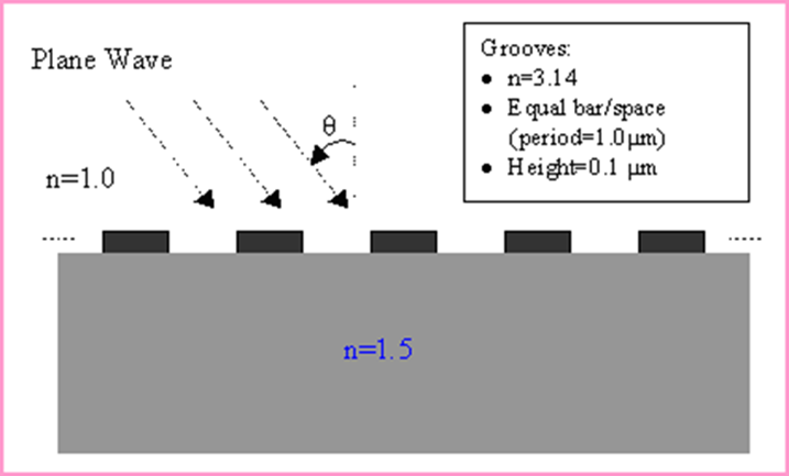
我們將模擬如圖1所示的二維光柵佈局。
圖1 二維光柵佈局
用VB腳本定義一個2D光柵佈局
步驟:
1. 通過在檔功能表中選擇“New”,啟動一個新專案。
2. 在“Wafer Properties”對話方塊中設置以下參數
Wafer Dimensions:
Length (mm): 8.5
Width (mm): 3.0
2D wafer properties:
Wafer refractive index: Air
3. 點擊 Profiles 與 Materials.
在“Materials”中加入以下材料:
Name: N=1.5
Refractive index (Re:): 1.5
Name: N=3.14
Refractive index (Re:): 3.14
4. 在“Profile”中定義以下輪廓:
Name: ChannelPro_n=3.14
2D profile definition, Material: n=3.14
Name: ChannelPro_n=1.5
2D profile definition, Material: n=1.5
6.畫出以下波導結構:
a. Linear waveguide 1
Label: linear1
Start Horizontal offset: 0.0
Start vertical offset: -0.75
End Horizontal offset: 8.5
End vertical offset: -0.75
Channel Thickness Tapering: Use Default
Width: 1.5
Depth: 0.0
Profile: ChannelPro_n=1.5
b. Linear waveguide 2
Label: linear2
Start Horizontal offset: 0.5
Start vertical offset: 0.05
End Horizontal offset: 1.0
End vertical offset: 0.05
Channel Thickness Tapering: Use Default
Width: 0.1
Depth: 0.0
Profile: ChannelPro_n=3.14
7. 加入水準平面波:
Continuous Wave Wavelength: 0.63 General:
Input field Transverse: Rectangular
X Position: 0.5
Direction: Negative Direction
Label: InputPlane1
2D Transverse:
Center Position: 4.5
Half width: 5.0
Titlitng Angle: 45
Effective Refractive Index: Local Amplitude: 1.0
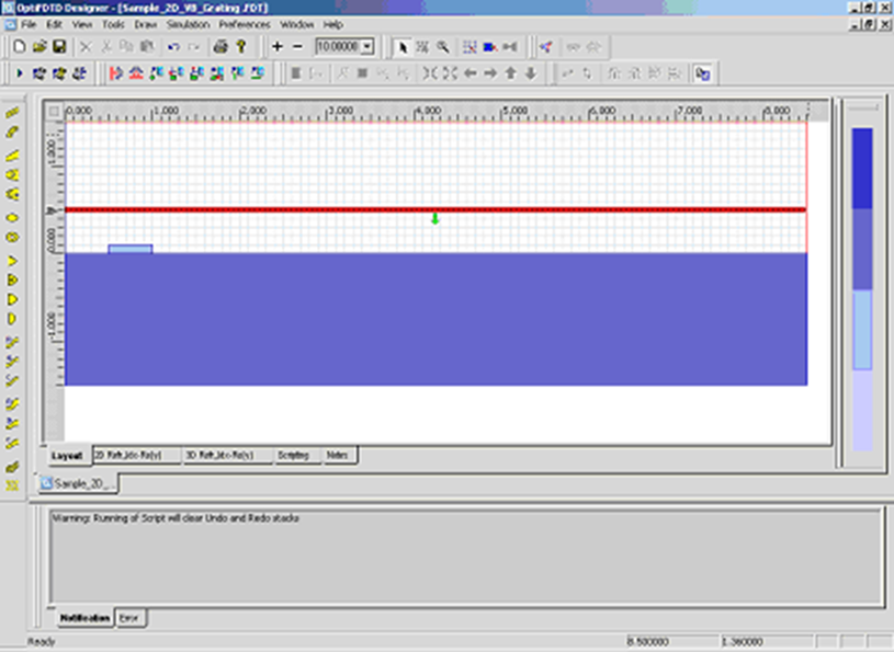
圖2 波導結構(未設置週期)
8. 按一下“Layout Script”快捷列或選擇模擬功能表下的“Generate Layout Script…”。這一步將把佈局對象轉換為VB腳本代碼。
將Linear2程式碼片段修改如下:
Dim Linear2
for m=1 to 8
Set Linear2 = WGMgr.CreateObj ( "WGLinear", "Linear2"+Cstr(m) )
Linear2.SetPosition 0.5+(m-1)*1.0, 0.05, 1+(m-1)*1.0, 0.05
Linear2.SetAttr "WidthExpr", "0.1"
Linear2.SetAttr "Depth", "0"
Linear2.SetAttr "StartThickness", "0.000000"
Linear2.SetAttr "EndThickness", "0.000000"
Linear2.SetProfileName "ChannelPro_n=3.14"
Linear2.SetDefaultThicknessTaperMode True
點擊“Test Script”快捷列運行修改後的VB腳本代碼。生成光柵佈局,佈局如圖3所示。
圖3光柵佈局通過VB腳本生成
設置模擬參數
1. 在Simulation功能表下選擇“2D simulation parameters…”,將出現模擬參數對話方塊
2. 在模擬參數對話方塊中,設置以下參數:
TE simulation
Mesh Delta X: 0.015
Mesh Delta Z: 0.015
Time Step Size: Auto Run for 1000 Time steps
設置邊界條件設置X和Z邊為各向異性PML邊界條件。
Number of Anisotropic PML layers: 15
其它參數保持默認
運行模擬
 在模擬參數中點擊Run按鈕,啟動模擬 在模擬參數中點擊Run按鈕,啟動模擬
在分析儀中,可以觀察到各場分量的時域回應
模擬完成後,點擊“Yes”,啟動分析儀。
遠場分析繞射波
1. 在OptiFDTD Analyzer中,在工具視窗中選擇“Crosscut Viewer”
2. 選擇“Definition of the Cross Cut”為z方向
3. 將位置移動到等於92的網格點,(位置:-0.12)觀察當前位置的近場
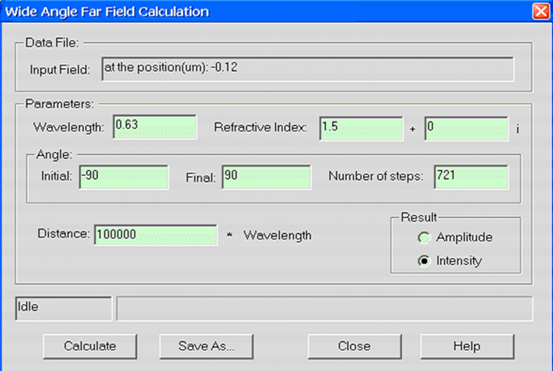
4. 在Crosscut Viewer的工具功能表中選擇“Far Field”,出現遠場轉換對話方塊。(圖4)
圖4 遠場計算對話方塊
5. 在遠場對話方塊,設置以下參數:
Wavelength: 0.63
Refractive index: 1.5+0i
Angle Initial: -90.0
Angle Final: 90.0
Number of Steps: 721
Distance: 100, 000*wavelength
Intensity
6. 點擊“計算”按鈕開始計算,並將結果保存為 Farfield.ffp。
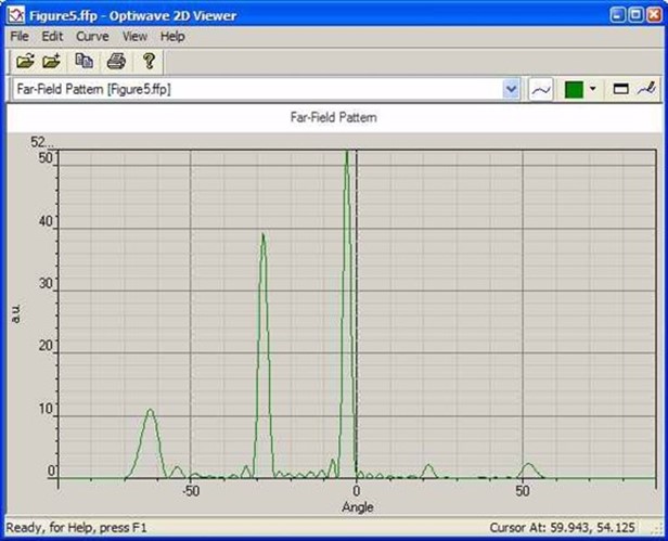
7. 啟動“Opti 2D Viewer”並載入Farfield.ffp。遠場如圖5所示。
圖5 “Opti 2D Viewer”中的遠場模式
|